Adaptive refinement and dynamic optimization

The parallelization approach described in the last two sections is well suited for fixed grids, which remain constant through all calculation steps. We will now introduce a simple, but effective method for an adaptive grid refinement and an improvement of the parallel algorithm which takes into account that the work load for each processor has changed after every refinement step. Before we can describe the algorithms, some questions have to be answered: what does refinement mean exactly, which parts should be refined, and how can we construct the new, refined grid.

• Refinement in our case means the splitting of elements into smaller elements, which replace the original elements.

• The question, which parts should be refined now turns into the selection of elements that should be refined. Therefore we choose for a given flow problem a characteristic function, e.g. the pressure field. We then look for elements, where the gradient of this function exceeds a given bound.

   
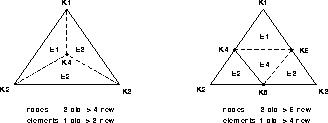
  Figure 5:   Splitting of an element
  

• How should these elements be split into smaller ones? In figure 5 two possibilities are shown: Using the left alternative leads to numerical problems, caused by the shape of the resulting triangles. Especially if an element is refined several times, the new grid nodes will be placed near to the remaining sides leading to very flat triangles, which should be avoided. So we must use the right alternative, which leads to the problem that the new nodes are placed on the edges of a triangle. This would result in an inconsistent grid, because all nodes must be corners of elements. The solution of this problem is an additional splitting of elements with such edges. Elements with two or three refined edges must be split into four elements (as if they where originally selected for refinement). Elements with only one refined edge must be split into two elements in a canonical way. This additional splitting of elements can lead to new elements with nodes on their edges, so the process has to be repeated until no more splitting is necessary.

• How can we construct the new grid? Every split element will be replaced by one of the new elements, the remaining new elements will be added to the element list. All new nodes are added to the node list and all new border nodes and elements are added to the appropriate lists. A new local time step for every element must be calculated and in the case of an instationary solution a new global time step must be calculated from the local time steps. After this some derived values like element sizes have to be reinitialized and then the calculations can continue.

Now we can formulate the refinement step:

 
  		calculate reference function F

  		Delta = (Max(F) - Min(F)) * refine_rate

  		for (El in element-list)

  				dF = local gradient of F in El

  				if (dF > Delta)

  						mark El with red

  				else

  						mark El with white

  				end-if

  		end-for

  		mark all elements with nodes on edges:

  				with yellow for full refinement

  				with green for half refinement

  		refine all elements full or half according to their colour

  		construct new node- and element-lists

  		reinitialize all dependent variables

All steps can be implemented straightforward with one exception: the colouring of the elements that must be refined to get a consistent grid. This can be done efficiently with the following recursive algorithm:

 
  		for (El in element-list)

  				if (El is marked red)

  						mark_neighbours(El)

  				end-if

  		end-for



  		mark_neighbours(El):

  				for (E in neighbour-elements(El))

  						if (E is marked white)

  								mark E with green

  						else if (E is marked green)

  								mark E with yellow

  								mark_neighbours(E)

  						end-if

  				end-for

  		end-mark_neighbours

To insert this refinement step in the parallel algorithm, we have to analyse the different parts for parallelism:

		 calculate reference function F

				local data, fully parallel, no communication

		 Delta = (Max(F) - Min(F)) * refine_rate

				local data, global min/max, mostly parallel, global communication

		 mark elements with red or white

				local data, fully parallel, no communication

		 mark additional elements with yellow or green

				global data, sequential, global communication (collection)

		 refinement of elements

				global data, sequential, global communication (broadcast)

		 construct new node- and element-lists

				local data, fully parallel, no communication

		 reinitialize all dependent variables

				local data, fully parallel, local communications

We can see that most of the parts can be performed in parallel with no or little communication. The only exception is the additional colouring of elements and the construction of new elements and nodes. These parts operate on global data structures, so that a parallel version of them must lead to a very high degree of global communication. As these parts need only very little of the time spent on the complete refinement step, we decided to keep this parts sequential. All necessary data is collected from one processor, the two steps are processed, and the resulting data is broadcasted to the appropriate processors.

For a typical flow calculation up to five refinement steps are sufficient in most cases, so that the lack of parallelism in the refinement step decribed above is not very problematic. Much more important is the fact that after a refinement step the work load of every processor has changed. As the refinement takes place in only small regions there are a few processors with a load that is much higher than the load of most of the other processors. This would not only slow down the calculations, but can lead to memory problems if further refinements in the same region take place. The solution of this problems is a dynamic load balancing, where parts of the sub grids are exchanged between processors until equal work load and nearly equal memory consumption is reached.

The load is obtained by simply measuring the CPU-time needed for one time step including communication times but excluding idle times. The items that could be exchanged between processors are single elements including their nodes and all the related data. To achieve this efficiently, we had to use dynamic data structures for all element and node data. There is one data block for every node and every element. These blocks are linked together in many different dynamic lists. The exchange of one element between two processors is therefore a complex operation: the element has to be removed from all lists on one processor and must be included in all lists on the other processor. Since nodes can be used on more than one processor, the nodes belonging to that element must not be exchanged in every case. It must be checked, whether they are already on the target processor and if other elements on the sending processor will need them, too. Nodes not availiable on the target processor must be sent to it and nodes which are no longer needed on the sending processor must be deleted there.

 
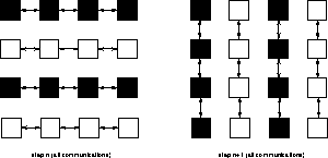
Figure 6:   Areas for dynamic load balancing

One remaining problem is to find an efficient strategy for the exchange of elements. A good strategy should deliver an even load balance after only a few steps and every step should be finished in a short time. As elements can only be exchanged between direct neighbours, a first approach was a local exchange between pairs of processors. This results in fast exchange steps, but shows a bad convergence behaviour. A global exchange would converge very fast, but at the cost of the lack of any parallelism. We will present here a semi-global strategy, where the balancing is carried out along the rows and columns of the processor grid. As shown in figure 6, the balancing areas are alternating all rows and all columns, where every row (column) is treated independent from all other rows (columns). A single row (column) is interpreted as a tree with the middle processor as the root and then we can use a modification of a tree balancing algorithm developed for combinatorical optimization problems [7].

This algorithm uses two steps: in a first step information about the local loads of the tree is moving up to the root and the computed optimal load value is propagated down the tree. In a second step the actual exchange is done according to the optimal loads found in the first step. The first step has the following structure, where num_procs is the number of processors in the tree (= row or column) and load_move_ direction is the load that has to be moved in that direction in the second step:

 
  		if (root)

  				receive load_sub_l (load of left subtree)

  				receive load_sub_r (load of right subtree)

  				global_load = local_load + loads of subtrees

  				load_opt = global_load / num_procs

  				send load_opt to subtrees

  				load_move_l = load_opt * num_sub_l - load_sub_l

  				load_move_r = load_opt * num_sub_r - load_sub_r

  		else

  				receive load_sub from subtree (if not leaf)

  				load_sub_n_me += load_sub

  				send load_sub_n_me to parent node

  				receive load_opt from parent node

  				send load_opt to subtree (if not leaf)

  				load_move_sub = load_opt * num_sub - load_sub

  				load_move_top = load_sub_n_me - (num_sub + 1) * load_opt

  		end-if

The second step is very simple: all processors translate the loads they have to move into the appropriate number of elements and exchange these elements. For the decision, which element to send in a specific direction, the virtual coordinates of this element are looked up and the element with the greatest value is choosen.