Figure 7: Different load balancing strategies
The algorithms described in the previous chapters were tested with a lot of different grids for various flow problems. As a kind of benchmark problem we use the instationary calculation of inviscid flow behind a cylinder, resulting in a vortex street. One grid for this problem was used for all our implementations of the parallel calculations. This grid has a size of about 12000 grid points which are forming nearly 20000 elements (P1). Other problems used with the adaptive refinement procedure are stationary turbine flows with grids of different sizes, all of them using periodic borders.

Figure 7: Different load balancing strategies
All measurements were made with a 1024 processor system located at the of the University of Paderborn. It consists of T805 Transputers, each of them equipped with 4 MByte local memory and coupled together as a two-dimensional grid. Our algorithms are all coded in Ansi-C using the Parix communication library.
First we will present some results for the dynamic load balancing. Figure 7 shows the different convergence behaviour of two different strategies. To investigate this, we used a start division of our reference problem with an extremely bad load balancing. The left picture shows the results of a local strategy, where the balance improves in the first steps, but stays away from the optimum for a large number of optimization steps. The right picture shows the effects of the described semi-global balancing, where after two steps the balance is nearly optimal.

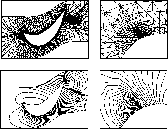
Figure 8: Grid and isobars after five refinement steps (complete and zoomed)
An example for the adaptive refinement procedure is shown in figure 8, where the grid and the pressure field around a turbine is shown after five refinement steps. One can see the high resolution of the two shocks made visible by the adaptive refinements. Without refinement one of these effects can only be guessed, the other is missing completely.

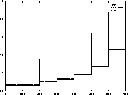
Figure 9: Load balancing for adaptive refinements
The development of the corresponding loads can be seen in figure 9. After each refinement step four balancing steps were carried out, using the semi-global strategy. The picture shows the efficient and fast balancing of this method.
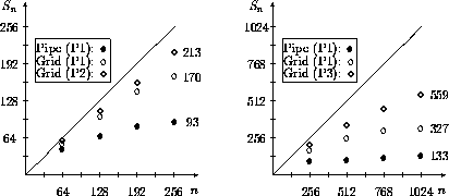
At last we will present results for large processor numbers. In figure 10 the speedups for some parameter settings of our reference problem are shown. In the speedup curves the difference between the logical topologies 1D-pipeline and 2D-grid is shown. In the left part of the picture we can see that for up to 256 processors we achieve nearly linear speedup with the grid topology, whereas the pipe topology is only linear for a maximum of 128 processors. If we increase the size of the problem (P2), the speedups are closer to the theoretical values, which proofs the scalability of the parallelization approach.

Figure 10: Speedups for different topologies
If we increase the number of processors (right picture) we observe that the grid topology again is superior to the pipe topology, but the increase of speedup is no longer linear. It is a common problem for most parallel algorithms that for a fixed problem size there is always a number of processors where the speedup is no longer increasing proportionally to the number of processors. If we want to get the same efficiencies as for 256 processors we have to use grids with approximately 50000 elements. This was impossible on the used T8-system, because such problems are too large for it. The biggest problem that fits into the 4 Mbyte nodes has about 32000 elements (P3), so that the speedups for 1024 processors are limited on this machine. Nevertheless, the increase of speedup to 559 shows the scalability of our algorithm again.